OPTIMIZER STATISTICS

 Optimizer statistics are a collection of data that describe the database and the objects in it. The optimizer uses these statistics to choose the best execution plan for each SQL statement. Being able to gather the appropriate statistics in a timely manner is critical to maintaining acceptable performance on any Oracle system. With each new release, Oracle strives to provide the necessary statistics automatically.

A summary is presented here, but full details can be found in Reference 1, Understanding Optimizer Statistics with Oracle Database 19c.

High-frequency Automatic Statistics Gathering

This Oracle Database 19c new feature is available on certain Oracle Database platforms. Check the Oracle Database Licensing Guide for more information.

Stale statistics can mislead the optimizer and in some cases can result in a sub-optimal plan. To address this, automatic optimizer statistics collection was introduced in Oracle 11g. The automated maintenance task infrastructure schedules statistics gathering to occur in maintenance windows. By default, one window is scheduled for each day of the week and statistics collection runs in all predefined maintenance windows.

For systems with rapidly changing datasets, data can drastically change in a short period time, rapidly rendering statistics stale and making daily statistics gathering insufficient.

New to Oracle Database 19c, high-frequency automatic statistics collection is introduced as a complement to the existing auto task. It is decoupled from the maintenance window. By configuring the DBMS_STATS preferences, the DBA can customize the frequency and maximum run time according to their requirement. Note that the existing automatic statistics collection running in the predefined maintenance window will not be affected, and high-frequency automatic statistics task will not start during the maintenance window.

Histograms

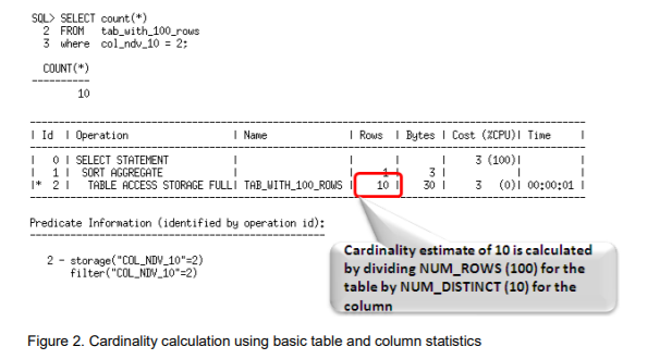
Histograms tell the optimizer about the distribution of data within a column. By default, the optimizer assumes a uniform distribution of rows across the distinct values in a column and will calculate the cardinality for a query with an equality predicate by dividing the total number of rows in the table by the number of distinct values in the column used in the equality predicate. The presence of a histogram changes the formula used by the optimizer to determine the cardinality estimate, and allows it to generate a more accurate estimate.

Online Statistics Gathering

When an index is created, Oracle automatically gathers optimizer statistics as part of the index creation by piggybacking the statistics gather on the full data scan and sort necessary for the index creation (this has been available since Oracle Database 9i). The same technique is applied for direct path operations such as, create table as select (CTAS) and insert as select (IAS) operations into empty tables. Piggybacking the statistics gather as part of the data loading operation, means no additional full data scan is required to have statistics available immediately after the data is loaded. The additional time spent on gathering statistics is small compared to a separate statistics collection process, and it guarantees to have accurate statistics readily available from the get-go.

Real-time Statistics

This Oracle Database 19c new feature is available on certain Oracle Database platforms. Check the Oracle Database Licensing Guide for more information.

Online statistics gathering for create table as select (CTAS) and direct path insert was first introduced in Oracle Database 12c Release 1. This allows statistics to be accurate and available immediately, but prior to Oracle Database 19c, this capability was not applicable to conventional database manipulation language (DML) operations which dominate the way data is manipulated in (for example) traditional OLTP systems.

Real-time statistics extends the online statistic gathering techniques to conventional insert, update and merge DML operations. In order to minimize the performance overhead of generating these statistics, only the most essential optimizer statistics are gathered during DML operations. The collection of the remaining stats (such as the number of distinct values) is deferred to the automatic statistics gathering job, high-frequency stats gathering and/or the manual invocation of the DBMS_STATS API. See Reference 2, Best Practices for Gathering Optimizer Statistics with Oracle Database 19c, for more information.

Incremental Statistics

Gathering statistics on partitioned tables consists of gathering statistics at both the table level (global statistics) and at the (sub)partition level. If data in (sub)partitions is changed in any way, or if partitions are added or removed, then the global-level statistics must be updated to reflect the changes so that there is correspondence between the partition-level and global-level statistics. For large partitioned tables, it can be very costly to scan the whole table to reconstruct accurate global-level statistics. For this reason, incremental statistics were introduced in Oracle Database 11g to address this issue, whereby synopses were created for each partition in the table. These data structures can be used to derive global-level statistics – including non-aggregatable statistics such as column cardinality - without scanning the entire table.

Incremental Statistics and Staleness

A DBMS_STATS preference called INCREMENTAL_STALENESS allows you to control when partition statistics will be considered stale and not good enough to generate global level statistics. By default, INCREMENTAL_STALENESS is set to NULL, which means partition level statistics are considered stale as soon as a single row changes (the same behavior as in Oracle Database 11g). Alternatively, it can be set to USE_STALE_PERCENT or USE_LOCKED_STATS. USE_STALE_PERCENT means the partition level statistics will be used as long as the percentage of rows changed (in the respective partition or subpartition) is less than the value of the preference STALE_PERCENTAGE (10% by default). USE_LOCKED_STATS means if statistics on a partition are locked, they will be used to generate global level statistics regardless of how many rows have changed in that partition since statistics were last gathered.

Incremental Statistics and Partition Exchange Loads

One of the benefits of partitioning is the ability to load data quickly and easily, with minimal impact on the business users, by using the exchange partition command. The exchange partition command allows the data in a non-partitioned table to be swapped into a specified partition in the partitioned table. The command does not physically move data; instead it updates the data dictionary to exchange a pointer from the partition to the table and vice versa.

The Oracle Database allows you to create the necessary statistics (synopses) on load tables before they are exchanged into the partitioned table. This means that global partition statistics can be maintained incrementally the moment that the load table is exchanged with the relevant table partition.

Compact Synopses

The performance for statistics gathering with incremental statistics can come with the price of high disk storage of synopses (they are stored in the SYSAUX tablespace). More storage is required for synopses for tables with a high number of partitions and a large number of columns, particularly where the number of distinct values (NDV) is high. Besides consuming storage space, the performance overhead of maintaining very large synopses can become significant. Oracle Database 12c Release 2 introduced a new algorithm for gathering and storing NDV information, which results in much smaller synopses while maintaining a similar level of accuracy to the previous algorithm.

CONCURRENT STATISTICS

When the global statistics gathering preference CONCURRENT is set, Oracle employs the Oracle Job Scheduler to create and manage one statistics gathering job per object (tables and / or partitions) concurrently.

AUTOMATIC COLUMN GROUP DETECTION

Extended statistics were introduced in Oracle Database 11g. They help the optimizer improve the accuracy of cardinality estimates for SQL statements that contain predicates involving a function wrapped column (e.g. UPPER(LastName)) or multiple columns from the same table that are used in filter predicates, join conditions, or group-by keys. Although extended statistics are extremely useful it can be difficult to know which extended statistics should be created if you are not familiar with an application or data set.

Auto column group detection, automatically determines which column groups are required for a table based on a given workload. The detection and creation of column groups is a simple three-step procedure3.

NEW REPORTING SUBPROGRAMS IN DBMS_STATS PACKAGE

Knowing when and how to gather statistics in a timely manner is critical to maintain acceptable performance on any system. Determining what statistics gathering operations are currently executing in an environment and how changes to the statistics methodology will impact the system can be difficult and time consuming.

Reporting subprograms in DBMS_STATS package make it easier to monitor what statistics gathering activities are currently going on and what impact changes to the parameter settings of these operations will have. The DBMS_STATS subprograms are REPORT_STATS_OPERATIONS, REPORT_SINGLE_STATS_OPERATION and REPORT_GATHER_*_STATS.

Figure 18 shows an example output from the REPORT_STATS_OPERATIONS function. The report shows detailed information about what statistics gathering operations have occurred, during a specified time window. It gives details on when each operation occurred, its status, and the number of objects covered and it can be displayed in either text or HTML format.

SQL plan directives

 SQL plan directives

SQL plan directives are automatically created based on information learnt via automatic re-optimization. A SQL plan directive is additional information that the optimizer uses to generate a more optimal execution plan. For example, when joining two tables that have a data skew in their join columns, a SQL plan directive can direct the optimizer to use dynamic statistics to obtain a more accurate join cardinality estimate.

SQL plan directives are created on query expressions rather than at a statement or object level to ensure they can be applied to multiple SQL statements. It is also possible to have multiple SQL plan directives used for a SQL statement. The number of SQL plan directives used for a SQL statement is shown in the note section under the execution plan (Figure 15).

Figure 15: The number of SQL plan directives used for a statement is shown in the note section under the plan

The database automatically maintains SQL plan directives and stores them in the SYSAUX tablespace. Any SQL plan directive that is not used after 53 weeks will be automatically purged. SQL plan directives can also be manually managed (altered or deleted) using the package DBMS_SPD but it is not possible to manually create a SQL plan directive. SQL plan directives can be monitored using the views DBA_SQL_PLAN_DIRECTIVES and DBA_SQL_PLAN_DIR_OBJECTS (See Figure 16).

Figure 16: Monitoring SQL plan directives automatically created based on information learnt via re-optimization

There a two types of SQL plan directive rows: DYNAMIC_SAMPLING and DYNAMIC_SAMPLING_RESULT. The dynamic sampling type tells the optimizer that when it sees this particular query expression (for example, filter predicates on country_id, cust_city, and cust_state_province being used together) it should use dynamic sampling to address the cardinality misestimate.

The dynamic sampling result type is present from Oracle Database 12c Release 2 onwards and signifies where results from dynamic sampling queries are stored in the SQL directive repository (instead of the Server Result Cache as used by Oracle Database 12c Release 1).

Figure 17: Dynamic sampling results stored in the SQL plan directive repository in Oracle Database 12c Release 2 onwards.

From Oracle Database 12c Release 2 onwards, SQL plan directives are created but they are not used at parse time to modify SQL execution plans. This prioritizes plan stability over maximizing query execute performance. The optimizer's use of SQL plan directives is controlled by the database initialization parameter optimizer_adaptive_statistics, which has the default value of FALSE. This setting is recommended for most systems.

In addition to finding optimal SQL execution plans, SQL plan directives can be used by the database to determine if extended statistics2, specifically column groups, are missing and would resolve the cardinality misestimates. After a SQL directive is used the optimizer decides if the cardinality misestimate could be resolved with a column group. If so, the database can automatically create that column group the next time statistics are gathered on the appropriate table. This step is “always on” in Oracle Database 12c Release 1, but from Oracle Database 12c Release 2, it is controlled by the DBMS_STATS preference AUTO_STAT_EXTENSIONS. The recommended (and default) value is OFF. This prioritizes plan stability over maximizing query performance. Automatic column group creation can be enabled using the following step:

EXEC DBMS_STATS.SET_GLOBAL_PREFS('AUTO_STAT_EXTENSIONS', 'ON')

Extended statistics will be used in place of the SQL plan directive when possible (equality predicates, group bys etc.). If the SQL plan directive is no longer necessary it will be automatically purged after 53 weeks.

re-optimization is Performance Feedback in Oracle

Performance Feedback

Another form of re-optimization is Performance Feedback, which helps to improve the degree of parallelism chosen for repeated SQL statements when Automatic Degree of Parallelism (Auto DOP)1 is enabled with parallel_degree_policy = ADAPTIVE.

When Auto DOP is enabled in adaptive mode, during the first execution of a SQL statement, the optimizer determines if the statement should execute in parallel and if so what parallel degree should be used. The parallel degree is chosen based on the estimated performance of the statement. Additional performance monitoring is also enabled for the initial execution of any SQL statement the optimizer decides to execute in parallel.

At the end of the initial execution, the parallel degree chosen by the optimizer is compared to the parallel degree computed base on the actual performance statistics (e.g. CPU-time) gathered during the initial execution of the statement. If the two values vary significantly then the statement is marked for re-optimization and the initial execution performance statistics are stored as feedback to help compute a more appropriate degree of parallelism for subsequent executions.

If performance feedback is used for a SQL statement then it is reported in the note section under the plan as shown in Figure 14.

Figure 14:

Statistics Feedback in Oracle

Statistics Feedback

Statistics feedback (formally known as cardinality feedback) is one form of re-optimization that automatically improves plans for repeated queries that have cardinality misestimates. During the first execution of a SQL statement, the optimizer generates an execution plan and decides if it should enable statistics feedback monitoring for the cursor. Statistics feedback is enabled in the following cases: tables with no statistics, multiple conjunctive or disjunctive filter predicates on a table, and predicates containing complex operators for which the optimizer cannot accurately compute cardinality estimates.

At the end of the execution, the optimizer compares its original cardinality estimates to the actual cardinalities observed during execution and, if estimates differ significantly from actual cardinalities, it stores the correct estimates for subsequent use. It will also create a SQL plan directive so other SQL statements can benefit from the information learnt during this initial execution. If the query executes again, then the optimizer uses the corrected cardinality estimates instead of its original estimates to determine the execution plan. If the initial estimates are found to be accurate no additional steps are taken. After the first execution, the optimizer disables monitoring for statistics feedback.

Figure 10 shows an example of a SQL statement that benefits from statistics feedback. On the first execution of this two-table join, the optimizer underestimates the cardinality by 8X due to multiple, correlated, single-column predicates on the customers table.

Where estimates vary greatly from the actual number of rows returned, the cursor is marked IS_REOPTIMIZIBLE and will not be used again. The IS_REOPTIMIZIBLE attribute indicates that this SQL statement should be hard parsed on the next execution so the optimizer can use the execution statistics recorded on the initial execution to determine a better execution plan.

A SQL plan directive is also created, to ensure that the next time any SQL statement that uses similar predicates on the customers table is executed, the optimizer will be aware of the correlation among these columns.

On the second execution the optimizer uses the statistics from the initial execution to determine a new plan that has a different join order. The use of statistics feedback in the generation of execution plan is indicated in the note section under the execution plan.

The new plan is not marked IS_REOPTIMIZIBLE, so it will be used for all subsequent executions of this SQL statement.

Figure 13:

ADAPTIVE STATISTICS and DYNAMIC STATISTICS

ADAPTIVE STATISTICS

The quality of the execution plans determined by the optimizer depends on the quality of the statistics available. However, some query predicates become too complex to rely on base table statistics alone and the optimizer can now augment these statistics with adaptive statistics.

The use of adaptive statistics can extend SQL statement parse times, which can become an overhead in systems that have high hard parse rates. In addition, SQL execution plans are likely to be more dynamic and less consistent. This feature is disabled by default from Oracle Database 12c Release 2 onwards. Systems that have low hard parse rates and complex queries (particularly ad-hoc queries) may benefit from this feature by setting the database initialization parameter optimizer_adaptive_statistics to TRUE.

DYNAMIC STATISTICS

During the compilation of a SQL statement, the optimizer decides if the available statistics are sufficient to generate a good execution plan or if it should consider using dynamic sampling. Dynamic sampling is used to compensate for missing or insufficient statistics that would otherwise lead to a very bad plan. For the case where one or more of the tables in the query does not have statistics, dynamic sampling is used by the optimizer to gather basic statistics on these tables before optimizing the statement. The statistics gathered in this case are not as high a quality (due to sampling) or as complete as the statistics gathered using the DBMS_STATS package.

Beginning with Oracle Database 12c Release 1, dynamic sampling was enhanced to become dynamic statistics. Dynamic statistics allow the optimizer to augment existing statistics to get more accurate cardinality estimates for not only single table accesses but also joins and group-by predicates. Also, from Oracle Database 12c Release 1, a new level 11 has been introduced for the initialization parameter OPTIMIZER_DYNAMIC_SAMPLING. Level 11 enables the optimizer to automatically decide to use dynamic statistics for any SQL statement, even if all basic table statistics exist. The optimizer bases its decision to use dynamic statistics on the complexity of the predicates used, the existing base statistics, and the total execution time expected for the SQL statement. For example, dynamic statistics will kick in for situations where the optimizer previously would have used a guess, such as queries with LIKE predicates and wildcards.

The default dynamic sampling level is 2, so it’s likely that when set to level 11, dynamic sampling will kick-in much more often and will increase hard parse times.

AUTOMATIC RE-OPTIMIZATION

During the first execution of a SQL statement, an execution plan is generated as usual. During optimization, certain types of estimates that are known to be of low quality (for example, estimates for tables which lack statistics or tables with complex predicates) are noted, and monitoring is enabled for the cursor that is produced. If feedback monitoring is enabled for a cursor by the system, cardinality estimates in the plan are compared to the actual cardinalities seen during execution. If estimates are found to differ significantly from the actual cardinalities, then the optimizer looks for a replacement plan on the next execution. The optimizer will use the information gathered during the previous execution to help determine an alternative plan. The optimizer can re-optimize a query several times, each time learning more and further improving the plan. Oracle Database 19c supports multiple forms of re-optimization.

ADAPTIVE QUERY OPTIMIZATION IN ORACLE

Adaptive Query Optimization is a set of capabilities that enable the optimizer to make run-time adjustments to execution plans and discover additional information that can lead to better statistics. 

This new approach is extremely helpful when existing statistics are not sufficient to generate an optimal plan. There are two distinct aspects in Adaptive Query Optimization: adaptive plans, which focuses on improving the execution of a query and adaptive statistics, which uses additional information to improve query execution plans.

Adaptive Plans

An adaptive plan will be chosen by the Optimizer if certain conditions are met; for example, when a query includes joins and complex predicates that make it difficult to estimate cardinality accurately. Adaptive plans enable the optimizer to defer the plan decision for a statement until execution time. The optimizer instruments its chosen plan (the default plan), with statistics collectors so that at runtime, it can detect if cardinality estimates differ greatly from the actual number of rows seen by the operations in the plan. If there is a significant difference, then the plan or a portion of it will be automatically adapted to avoid suboptimal performance.

From Oracle Database 12.2 onwards, adaptive plans are enabled and disabled using the database parameter optimizer_adaptive_plans. Use of the default value of TRUE (enabled) is recommended.

ADAPTIVE JOIN METHODS

The optimizer is able to adapt join methods on the fly by predetermining multiple sub-plans for portions of the plan. For example, in Figure 3, the optimizer’s default plan choice for joining the orders and products tables is a nested loops join via an index access on the products table. An alternative sub-plan, has also been determined that allows the optimizer to switch the join type to a hash join. In the alternative plan the products table will be accessed via a full table scan.

During the initial execution, the statistics collector gathers information about the execution and buffers a portion of rows coming into the sub-plan. The Optimizer determines what statistics are to be collected, and how the plan should be resolved for different values of the statistics. It computes an “inflection point” which is the value of the statistic where the two plan choices are equally good. For instance, if the nested loops join is optimal when the scan of an orders table produces fewer than 10 rows, and the hash join is optimal when the scan of orders produces more than 10 rows, then the inflection point for these two plans is 10. The optimizer computes this value, and configures a buffering statistics collector to buffer and count up to 10 rows. If at least 10 rows are produced by the scan, then the join method is resolved to hash join; otherwise it is resolved to nested loops join. In Figure 3, the statistics collector is monitoring and buffering rows coming from the full table scan of orders. Based on the information seen in the statistics collector, the optimizer will make the decision about which sub-plan to use. In this case, the hash join is chosen since the number of rows coming from the orders table is larger than the optimizer initially estimated.

The optimizer can switch from a nested loops join to a hash join and vice versa. However, if the initial join method chosen is a sort merge join no adaptation will take place.

By default, the explain plan command will show only the initial or default plan chosen by the optimizer. Whereas the DBMS_XPLAN.DISPLAY_CURSOR function displays the plan actually used by the query.

To see all of the operations in an adaptive plan, including the positions of the statistics collectors, the additional format parameter ‘adaptive’ must be specified in the DBMS_XPLAN functions. In this mode, an additional notation “-” appears in the Id column of the plan, indicating the operations in the plan that were not used (inactive).

SQL Monitor visualizes all operations if “Full” is selected in the “Plan” drop down box. The inactive parts of the plan are grayed out (see Figure 6). If the “Plan Note” icon is clicked, a pop-up box will be displayed confirming that the plan is an adaptive plan.

ADAPTIVE PARALLEL DISTRIBUTION METHODS

When a SQL statement is executed in parallel certain operations, such as sorts, aggregations, and joins require data to be redistributed among the parallel server processes executing the statement. The distribution method chosen by the optimizer depends on the operation, the number of parallel server processes involved, and the number of rows expected. If the optimizer inaccurately estimates the number of rows, then the distribution method chosen could be suboptimal and could result in some parallel server processes being underutilized.

With the new adaptive distribution method, HYBRID HASH the optimizer can defer its distribution method decision until execution, when it will have more information on the number of rows involved. A statistics collector is inserted before the operation and if the actual number of rows buffered is less than the threshold the distribution method will switch from HASH to BROADCAST. If however the number of rows buffered reaches the threshold then the distribution method will be HASH. The threshold is defined as 2 X degree of parallelism.

Figure 7 shows an example of a SQL Monitor execution plan for a join between EMP and DEPT that is executed in parallel. One set of parallel server processes (producers or pink icons) scan the two tables and send the rows to another set of parallel server processes (consumers or blue icons) that actually do the join. The optimizer has decided to use the HYBRID HASH distribution method. The first table accessed in this join is the DEPT table. The rows coming out of the DEPT table are buffered in the statistics collector, on line 6 of the plan, until the threshold is exceeded or the final row is fetched. At that point the optimizer will make its decision on a distribution method.

To understand which distribution method was chosen at runtime, the easiest way to find this information is to look at the OTHER column in SQL Monitor. This column shows a binocular icon in the lines with PX SEND HYBRID HASH row source. When you click the icon, you can see the distribution method used at runtime.

For the adaptive distribution methods there are three possible values reported in this dialog box: 6 = BROADCAST, 5 = ROUND-ROBIN, and 16 = HASH distribution.

ADAPTIVE BITMAP INDEX PRUNING

When the optimizer generates a star transformation plan, it must choose the right combination of bitmap indexes to reduce the relevant set of ROWIDs as efficiently as possible. If there are many indexes, some of them might not reduce the ROWID set very substantially but will nevertheless introduce significant processing cost during query execution. Adaptive plans are therefore used to prune out indexes that are not significantly filtering down the number of matched rows.

DBMS_XPLAN.DISPLAY_CURSOR will reveal adaptive bitmap pruning in a SQL execution plan with the adaptive keyword in a similar manner to the example shown in Figure 4. For example, consider the following SQL execution plan showing the bitmap index CAR_MODEL_IDX being pruned:

AUTOMATIC INDEXING IN ORACLE

INDEXING CHALLENGES

Indexes are useful for most types of workload and particularly critical for high performance in online transaction processing (OLTP) and operational data store (ODS) environments. However, identifying the best indexes is not straightforward and can require a considerable amount of manual labor. This is largely because index management is a continuous process. Applications are rarely static; they change in response to changing business requirements. For this reason, there will be changes in data volumes, of course, but also less obvious changes in data value distributions and the way data is organized, processed and accessed.

Traditionally, DBAs have been responsible to monitoring performance and deciding when and where to add, change or remove indexes in a tactical and often ad-hoc manner. This ad-doc approach to index maintenance is prone to error because it is almost impossible to quantify the effect any change – both positive and negative. This may lead to a database that has many more indexes than necessary, where indexes have been gradually added over time and there is a reluctance to remove any of them for fear of negative consequences. This will lead to an increase the system resources required to maintain indexes when data is modified and processed. In addition, over-indexed environments often suffer from less stable SQL execution plans as the sheer number of indexes make the optimizer's choice of index access path more and more finely balanced.

AUTOMATIC INDEXING

Automatic indexing addresses these issues. It is not a simple advisor, but instead it is an expert system that implements indexes based on what a performance engineer skilled in index tuning would do. The Oracle Database analyzes the application workload and identifies the queries that will benefit from additional indexes. In other words, it identifies candidate indexes and validates them before implementation, and the entire process is fully automatic.

Here is a summary of the workflow:

The steps can be summarized as follows:

Capture

 Periodically capture SQL statements from the application workload in a SQL tuning set. This tuning set called the automatic SQL tuning set (ASTS).

Identify

 Identify candidate indexes that may benefit the application workload.

 Creates unusable and invisible index candidates (this is a data dictionary metadata change only)

Verify

 The optimizer verifies which index candidates will be used by the captures SQL statements

 Materialize the successful candidates and measure their effect on the performance of the captured 

SQL statements

 The indexes remain invisible to the application workload and all verification is done outside the application workflow

Decide

 Indexes that are found to offer a significant performance improvement are made visible to the application workload.

 Indexes that are found to provide insufficient performance benefits remain invisible to the application workload.

 Automatic indexing offers a mixed solution where necessary. If there is an overall benefit in using a particular auto-index, then it will be marked visible. If individual queries suffer from a performance regression, SQL plan baselines are used to prevent them from using regressed plans.

Monitor

 SQL performance and index usage is continuously monitored. Indexes that have not been used for a configurable period of time will be dropped.

Configuring and Monitoring Automatic Indexing

Automatic indexing requires little to no manual intervention, but a package called DBMS_AUTO_INDEX package is provided for changing a small number of defaults. The feature can be enabled as follows:

SQL> exec dbms_auto_index.configure('AUTO_INDEX_MODE', 'IMPLEMENT')

And disabled:

SQL> exec dbms_auto_index.configure('AUTO_INDEX_MODE', 'OFF')

The number of days unused auto-indexes are retained is controlled as follows:

SQL> exec dbms_auto_index.configure('AUTO_INDEX_RETENTION_FOR_AUTO', '373')

It is possible to specify which schemas are subject to auto indexing:

SQL> -- Exclude SH and HR

SQL> exec dbms_auto_index.configure('AUTO_INDEX_SCHEMA', 'SH', FALSE)

SQL> exec dbms_auto_index.configure('AUTO_INDEX_SCHEMA', 'HR', FALSE)

SQL> -- Remove HR from exclusion list

SQL> exec dbms_auto_index.configure('AUTO_INDEX_SCHEMA', 'HR', NULL)

SQL> -- Remove all schemas from exclusion list

SQL> exec dbms_auto_index.configure('AUTO_INDEX_SCHEMA', NULL, TRUE)

SQL> -- Include SH for auto indexing but exclude HR

SQL> exec dbms_auto_index.configure('AUTO_INDEX_SCHEMA', 'SH', FALSE)

SQL> exec dbms_auto_index.configure('AUTO_INDEX_SCHEMA', 'HR', TRUE)

All parameter settings (and schemas that have been included and excluded) can be seen as follows:

SQL> select * from dba_auto_index_config;

A report on auto index activity can be generated. 

For example:

SQL> set linesize 300 trims on pagesize 1000 long 100000

SQL> column report format a120

SQL> SELECT dbms_auto_index.report_activity(sysdate-30,null,'text','all','all') report FROM dual;

Here is an extract from an example report:

REPORT

------------------------------------------------------------------------------------------------------------------------

GENERAL INFORMATION

-------------------------------------------------------------------------------

Activity start : 29-DEC-2018 05:09:37

Activity end : 28-JAN-2019 05:09:37

Executions completed : 743

Executions interrupted : 0

Executions with fatal error : 0

-------------------------------------------------------------------------------

SUMMARY (AUTO INDEXES)

-------------------------------------------------------------------------------

Index candidates : 16

Indexes created (visible / invisible) : 2 (2 / 0)

Space used (visible / invisible) : 268.44 MB (268.44 MB / 0 B)

Indexes dropped : 0

SQL statements verified : 6

SQL statements improved (improvement factor) : 3 (493.3x)

SQL plan baselines created : 0

Overall improvement factor : 247.4x

-------------------------------------------------------------------------------

SUMMARY (MANUAL INDEXES)

-------------------------------------------------------------------------------

Unused indexes : 0

Space used : 0 B

Unusable indexes : 0

-------------------------------------------------------------------------------

INDEX DETAILS

-------------------------------------------------------------------------------

1. The following indexes were created:

*: invisible

-------------------------------------------------------------------------------

----------------------------------------------------------------------

| Owner | Table | Index | Key | Type | Properties |

----------------------------------------------------------------------

| AUTOI | FACT1 | SYS_AI_0rn9u2kmxxbs7 | F1 | B-TREE | NONE |

| AUTOI | FACT1 | SYS_AI_151bnmf3xsxaw | F2,F3 | B-TREE | NONE |

----------------------------------------------------------------------

-------------------------------------------------------------------------------

VERIFICATION DETAILS

-------------------------------------------------------------------------------

1. The performance of the following statements improved:

-------------------------------------------------------------------------------

Parsing Schema Name : AUTOI

SQL ID : 34xymh9usuxzz

SQL Text : select /* TESTQ3 */ sum(f4) from fact1 where f1 = 10

Improvement Factor : 2268.9x

PLANS SECTION

---------------------------------------------------------------------------------------------

- Original

-----------------------------

Plan Hash Value : 4087791341

Histograms in Oracle

###########

Histograms

###########

A histogram is a special type of column statistic that provides more detailed information about the data distribution in a table column.

What are Histograms?

-----------------------------

> Holds data about values within a column in a table for the number of occurrences for a specific value/range.

> Used by CBO to optimize a query to use whatever index Fast Full scan or table full scan.

> Usually being used against columns have data being repeated frequently like country or city column.

> gathering histograms on a column having distinct values (PK) is useless because values are not repeated.

> Two types of Histograms can be gathered:

  -Frequency histograms are when distinct values (buckets) in the column is less than 255 (e.g. the number of countries is always less than 254).

  -Height balanced histograms: are similar to frequency histograms in their design, but distinct values bigger than 254.

> Collected by DBMS_STATS (which by default doesn't collect histograms, it deletes them if you didn't use the parameter).

> Mainly being gathered on foreign key columns/columns in WHERE statement.

> Help in SQL multi-table joins.

> Column histograms like statistics are being stored in the data dictionary.

> If the application is exclusive uses bind variables, Oracle recommends deleting any existing histograms and disabling Oracle histograms generation.

Cautions:

   – Do not create histograms on Columns that are not being queried.

   – Do not create histograms on every column of every table.

   – Do not create histograms on the primary key column of a table.

Verify the existence of histograms:

---------------------------------------------

SQL> select column_name,histogram from dba_tab_col_statistics

     where owner='SCOTT' and table_name='EMP'; 

Creating Histograms:

---------------------------

e.g.

SQL> Exec dbms_stats.gather_schema_stats

     (ownname => 'SCOTT',

     estimate_percent => dbms_stats.auto_sample_size,

     method_opt => 'for all columns size auto',

     degree => 7);

method_opt:

FOR COLUMNS SIZE AUTO                 => Fastest. you can specify one column instead of all columns.

FOR ALL COLUMNS SIZE REPEAT     => Prevent deletion of histograms and collect it only for columns already have histograms.

FOR ALL COLUMNS => collect histograms on all columns.

FOR ALL COLUMNS SIZE SKEWONLY => collect histograms for columns have skewed value.

FOR ALL INDEXES COLUMNS      => collect histograms for columns have indexes.

Note: AUTO & SKEWONLY will let Oracle decide whether to create the Histograms or not.

Check the existence of Histograms:

SQL> select column_name, count(*) from dba_tab_histograms

     where OWNER='SCOTT' table_name='EMP' group by column_name; 

Drop Histograms: 11g

----------------------

e.g.

SQL> Exec dbms_stats.delete_column_stats

     (ownname=>'SH', tabname=>'SALES',

     colname=>'PROD_ID', col_stat_type=> HISTOGRAM);

Stop gather Histograms: 11g

------------------------------

[This will change the default table options]

e.g.

SQL> Exec dbms_stats.set_table_prefs

     ('SH', 'SALES','METHOD_OPT', 'FOR ALL COLUMNS SIZE AUTO,FOR COLUMNS SIZE 1 PROD_ID');

>Will continue to collect histograms as usual on all columns in the SALES table except for PROD_ID column.

Drop Histograms: 10g

----------------------

e.g.

SQL> exec dbms_stats.delete_column_stats(user,'T','USERNAME');

Link:

https://docs.oracle.com/en/database/oracle/oracle-database/19/tgsql/histograms.html

Have you ever wondered how does Oracle determine what type of histograms to create?

As of 12c there are 4 types of histograms. Are you familiar with these types? How does Oracle decide which ones to choose out of the four?

• frequency
• top frequency
• height balanced
• hybrid

If you need an introduction to histograms, you can check out last week’s post: Intro To Histograms. Three Basic Questions Answered.

Let me first introduce you to each type of histogram, so you have a better understanding.

Frequency Histograms

If the histogram on your column is a frequency histogram, this means that there is a bucket for each distinct value of the column.
Here is an example:

You have the column COLOR, with 4 distinct values: red, blue, green, yellow. Let’s say there are 100 rows in the table that have the color red, 50 rows in the table that have the color blue, 10 rows in the table that have the color green, and 2 rows in the table that have the color yellow.

In this case, there will be 4 buckets in the histogram (one for each distinct value), red bucket with 100 values, blue bucket with 50 values, green bucket with 10 values, and the yellow bucket with 2 values.

For frequency histograms, each bucket can have a different number of values in it, which means some buckets could be more full than others.

Top Frequency Histograms

These type of histograms were introduced with 12c, and are similar to the frequency histograms. The difference is that the top frequency histograms ignore non-popular values that are statistically insignificant.
Let’s look at an example.
We have the column CITY, which has 300 distinct values for table A. This table A has 100,000 rows.
There are 20,000 rows with the column CITY as Toronto, 30,000 rows with the column CITY as Vancouver, 35,000 rows with the column CITY as Calgary. The rest of the 15,000 rows are divided between the rest of the 297 distinct values. However there are a few city values, such as Airdrie and Kelowna with 5 values each.
These 2 values will be considered non-popular values, and will be ignored (there will be no bucket for them).

Height-Balanced Histograms

The Height-Balanced Histograms are legacy type histograms. The column values are divided into buckets, and each bucket contains approximately the same number of rows. These type of histograms are not very “popular” in 12c and up.

Hybrid Histograms

These types of histograms were also introduced with 12c. They are a combination of height-balanced histograms and frequency histograms.
Oracle says it is the “best of both worlds”.

If you want to check whether or not a histogram exists on the columns of a table, query DBA_TAB_COL_STATISTICS.

SQL> select COLUMN_NAME,NUM_DISTINCT,NUM_BUCKETS,HISTOGRAM 
     from DBA_TAB_COL_STATISTICS 
     where table_name='A' and owner='DR' 
     order by column_name;

COLUMN_NAME      NUM_DISTINCT NUM_BUCKETS HISTOGRAM
---------------- ------------ ----------- ---------------
COL_1                     674         254 HYBRID
COL_2                       5           5 FREQUENCY
COL_3                       8           1 NONE
COL_4                    1348           1 NONE
COL_5                    1361         254 HYBRID
COL_6                    1346         254 HYBRID
COL_7                     299         254 TOP-FREQUENCY
COL_8                       5           5 FREQUENCY

8 rows selected.

If you want more information about the histogram itself that you have on a specific column, you can further query DBA_HISTOGRAMS view.
Be aware that there will be one row for each bucket of a histogram in the table:

SQL> select column_name, count(*) 
     from DBA_HISTOGRAMS 
     where table_name='A' and owner='DR' 
     group by column_name 
     order by column_name;

COLUMN_NAME     COUNT(*)
--------------- --------
COL_1                254
COL_2                  5
COL_3                  2
COL_4                  2
COL_5                254
COL_6                254
COL_7                254
COL_8                  5

8 rows selected.

In the above examples, have you noticed that:

• for frequency histograms, the number of distinct values is equal to the number of buckets.
• for hybrid histograms the number of distinct values is always greater than the number of buckets.
• for top-frequency histograms the number of distinct values is always greater than the number of buckets.

Also have you noticed that the maximum number if buckets is 254? You could have more buckets, however this is the default number of buckets that Oracle is using. If you do not specify explicitly the number of buckets when gathering stats, then by default the number of buckets is 254.

The height balanced histograms are not very common in 12c and up. Just running a quick select statement in my 12.1 environment, will prove that I have 0 histogram of type height balanced:

SQL> select count(*), histogram 
     from DBA_TAB_COL_STATISTICS group by histogram;

  COUNT(*) HISTOGRAM
---------- ---------------
       799 FREQUENCY
        71 HYBRID
         2 TOP-FREQUENCY
     32689 NONE

Now that you have a better understanding about histogram types, let’s explore how will Oracle decide which type of histograms to use.

Oracle is using 4 variables to determine the type of histogram to use. These variables are listed below:

1) number of distinct values in the column -> NDV. If the column in the table has the values red, blue, yellow, green, then NDV=4

2) number of histogram buckets -> n. The default value for n is 254. If you don’t explicitly specify the number of buckets, then by default Oracle will set the number of buckets to 254.

3) internal variable, percentage threshold, p = (1–(1/n)) * 100; This is a formula set by Oracle.

4) the value of estimate_percent, when you gather statistics, whether or not it’s set to default value AUTO_SAMPLE_SIZE, when gathering statistics.

👉Here are the rules, set by Oracle when picking a specific type of histogram:

Oracle will pick a Frequency Histogram if:
NDV < n (n=254 by default)
if number of distinct values is less than the number of histogram buckets.

Oracle will pick a Height Balanced Histogram if:
NDV > n (n=254 by default)
estimate_percent < > AUTO_SAMPLE_SIZE
if number of distinct values is greater than the number of histogram buckets
and the estimate percent is not set to AUTO_SAMPLE_SIZE during stats gathering.

Oracle will pick a Hybrid Histogram if:
NDV > n (n=254 by default)
estimate_percent = AUTO_SAMPLE_SIZE
percentage of rows for top n (n=254 by default) frequent values < p
If n=254, then p is 99.6

Oracle will pick a Top Frequency Histogram if
NDV > n (n=254 by default)
estimate_percent = AUTO_SAMPLE_SIZE
percentage of rows for top n (n=254 by default) frequent values >= p

Fixed OBJECTS, SYSTEM and Data Dictionary Statistics in Oracle

####################

Fixed OBJECTS Statistics

####################

What are Fixed objects:

----------------------------

-Fixed objects are the x$ tables (been loaded in SGA during startup) on which V$ views are built (V$SQL etc.).

-If the statistics are not gathered on fixed objects, the Optimizer will use predefined default values for the statistics. These defaults may lead to inaccurate execution plans.

-Statistics on fixed objects are not being gathered automatically or within gathering DB stats.

How frequent to gather stats on fixed objects?

-------------------------------------------------------

Only one time for a representative workload, but it's recommended to gather it whenever you hit one of the following events:

- After a major database or application upgrade.

- After implementing a new module.

- After changing the database configuration. e.g. changing the size of memory pools (sga, pga,..).

- Poor performance/Hang encountered while querying dynamic views e.g. V$ views.

Please note that:

- It's recommended to Gather the fixed object stats during peak hours (whilst the system is busy) or after the peak hours but the sessions are still connected (even if they idle), this will guarantee the population of new statistics representing the actual/average DB load.

- Performance degradation can happen during the gather of fixed objects statistics.

- Having no statistics (or using RULE Based Optimizer against fixed objects) is better than having a non-representative statistics on fixed objects.

How to gather stats on fixed objects:

---------------------------------------------

First Check the last analyzed date:

------ -----------------------------------

SQL> select OWNER, TABLE_NAME, LAST_ANALYZED

        from dba_tab_statistics where table_name='X$KGLDP'; 

Second Export the current fixed stats in a table: (in case you need to revert back)

------- -----------------------------------

SQL> EXEC DBMS_STATS.CREATE_STAT_TABLE

        ('OWNER','STATS_TABLE_NAME','TABLESPACE_NAME');

SQL> EXEC dbms_stats.export_fixed_objects_stats

        (stattab=>'STATS_TABLE_NAME',statown=>'OWNER'); 

Third Gather the fixed objects stats:

-------  ------------------------------------

SQL> exec dbms_stats.gather_fixed_objects_stats; 

Note:

New gathered statistics may not immediately take effect unless you flush the shared pool or restart the database.

In case you experienced a bad performance on fixed tables after the new statistics, simply restore back the statistics from the export you have done in step2:

SQL> exec dbms_stats.delete_fixed_objects_stats(); 

SQL> exec DBMS_STATS.import_fixed_objects_stats

        (stattab =>'STATS_TABLE_NAME',STATOWN =>'OWNER');

#################

SYSTEM STATISTICS

#################

What is system statistics:

-------------------------------

System statistics are statistics about CPU speed and IO performance, it enables the CBO to

effectively cost each operation in an execution plan. Introduced in Oracle 9i.

Why gathering system statistics:

----------------------------------------

Oracle highly recommends gathering system statistics during a representative workload,

ideally at peak workload time, in order to provide more accurate CPU/IO cost estimates to the optimizer.

You only have to gather system statistics once.

There are two types of system statistics (NOWORKLOAD statistics & WORKLOAD statistics):

NOWORKLOAD statistics:

-----------------------------------

This will simulate a workload -not the real one but a simulation- and will not collect full statistics, it's less accurate than "WORKLOAD statistics" but if you can't capture the statistics during a typical workload you can use no-workload statistics.

To gather noworkload statistics:

SQL> execute dbms_stats.gather_system_stats(); 

WORKLOAD statistics:

-------------------------------

This will gather statistics during the current workload [which supposed to be representative of the actual system I/O and CPU workload on the DB].

To gather WORKLOAD statistics:

SQL> execute dbms_stats.gather_system_stats('start');

Once the workload window ends after 1,2,3.. hours or whatever, stop the system statistics gathering:

SQL> execute dbms_stats.gather_system_stats('stop');

You can use time interval (minutes) instead of issuing start/stop command manually:

SQL> execute dbms_stats.gather_system_stats('interval',60); 

Check the system values collected:

-------------------------------------------

col pname format a20

col pval2 format a40

select * from sys.aux_stats$; 

cpuspeedNW:  Shows the noworkload CPU speed, (average number of CPU cycles per second).

ioseektim:    The sum of seek time, latency time, and OS overhead time.

iotfrspeed:  I/O transfer speed, tells optimizer how fast the DB can read data in a single read request.

cpuspeed:      Stands for CPU speed during a workload statistics collection.

maxthr:          The maximum I/O throughput.

slavethr:      Average parallel slave I/O throughput.

sreadtim:     The Single Block Read Time statistic shows the average time for a random single block read.

mreadtim:     The average time (seconds) for a sequential multiblock read.

mbrc:             The average multiblock read count in blocks.

Notes:

-When gathering NOWORKLOAD statistics it will gather (cpuspeedNW, ioseektim, iotfrspeed) system statistics only.

-Above values can be modified manually using DBMS_STATS.SET_SYSTEM_STATS procedure.

-According to Oracle, collecting workload statistics doesn't impose an additional overhead on your system.

Delete system statistics:

------------------------------

SQL> execute dbms_stats.delete_system_stats();

####################

Data Dictionary Statistics

####################

Facts:

-------

> Dictionary tables are the tables owned by SYS and residing in the system tablespace.

> Normally data dictionary statistics in 9i is not required unless performance issues are detected.

> In 10g Statistics on the dictionary tables will be maintained via the automatic statistics gathering job run during the nightly maintenance window.

If you choose to switch off that job for application schema consider leaving it on for the dictionary tables. You can do this by changing the value of AUTOSTATS_TARGET from AUTO to ORACLE using the procedure:

SQL> Exec DBMS_STATS.SET_PARAM(AUTOSTATS_TARGET,'ORACLE');  

When to gather Dictionary statistics:

---------------------------------------------

-After DB upgrades.

-After the creation of a new big schema.

-Before and after big datapump operations.

Check last Dictionary statistics date:

---------------------------------------------

SQL> select table_name, last_analyzed from dba_tables

     where owner='SYS' and table_name like '%$' order by 2; 

Gather Dictionary Statistics:  

-----------------------------------

SQL> EXEC DBMS_STATS.GATHER_DICTIONARY_STATS;

->Will gather stats on 20% of SYS schema tables.

or...

SQL> EXEC DBMS_STATS.GATHER_SCHEMA_STATS ('SYS');

->Will gather stats on 100% of SYS schema tables.

or...

SQL> EXEC DBMS_STATS.GATHER_DATABASE_STATS(gather_sys=>TRUE);

->Will gather stats on the whole DB+SYS schema.

################

Extended Statistics "11g onwards"

################

Extended statistics can be gathered on columns based on functions or column groups.

Gather extended stats on column function:

====================================

If you run a query having in the WHERE statement a function like upper/lower the optimizer will be off and index on that column will not be used:

SQL> select count(*) from EMP where lower(ename) = 'scott'; 

In order to make optimizer work with function-based terms you need to gather extended stats:

1-Create extended stats:

>>>>>>>>>>>>>>>>>>>>

SQL> select dbms_stats.create_extended_stats('SCOTT','EMP','(lower(ENAME))') from dual;

2-Gather histograms:

>>>>>>>>>>>>>>>>>

SQL> exec dbms_stats.gather_table_stats('SCOTT','EMP', method_opt=> 'for all columns size skewonly');

OR

----

*You can do it also in one Step:

>>>>>>>>>>>>>>>>>>>>>>>>>

SQL> Begin dbms_stats.gather_table_stats

     (ownname => 'SCOTT',tabname => 'EMP',

     method_opt => 'for all columns size skewonly for

     columns (lower(ENAME))');

     end;

     /

To check the Existence of extended statistics on a table:

----------------------------------------------------------------------

SQL> select extension_name,extension from dba_stat_extensions where owner='SCOTT'and table_name = 'EMP';

SYS_STU2JLSDWQAFJHQST7$QK81_YB (LOWER("ENAME"))

Drop extended stats on column function:

------------------------------------------------------

SQL> exec dbms_stats.drop_extended_stats('SCOTT','EMP','(LOWER("ENAME"))');

Gather extended stats on column group: -related columns-

=================================

Certain columns in a table that are part of a join condition (where statements are correlated e.g.(country, state). You want to make the optimizer aware of this relationship between two columns and more instead of using separate statistics for each column. By creating extended statistics on a group of columns, the Optimizer can determine a more accurate the relation between the columns are used together in a where clause of a SQL statement. e.g. columns like country_id and state_name the have a relationship, state like Texas can only be found in the USA so the value of state_name is always influenced by country_id.

If there are extra columns are referenced in the "WHERE statement with the column group the optimizer will make use of column group statistics.

1- create a column group:

>>>>>>>>>>>>>>>>>>>>>

SQL> select dbms_stats.create_extended_stats('SH','CUSTOMERS', '(country_id,cust_state_province)')from dual;

2- Re-gather stats|histograms for table so optimizer can use the newly generated extended statistics:

>>>>>>>>>>>>>>>>>>>>>>>

SQL> exec dbms_stats.gather_table_stats ('SH','customers',method_opt=> 'for all columns size skewonly');

OR

---

*You can do it also in one Step:

>>>>>>>>>>>>>>>>>>>>>>>>>

SQL> Begin dbms_stats.gather_table_stats

     (ownname => 'SH',tabname => 'CUSTOMERS',

     method_opt => 'for all columns size skewonly for

     columns (country_id,cust_state_province)');

     end; 

     /

Drop extended stats on column group:

--------------------------------------------------

SQL> exec dbms_stats.drop_extended_stats('SH','CUSTOMERS', '(country_id,cust_state_province)');

Optimizer Statistics in Oracle

What are Optimizer Statistics? 

Optimizer statistics are a collection of data that describe the database, and the objects in the database. These statistics are used by the Optimizer to choose the best execution plan for each SQL statement. 

Statistics are stored in the data dictionary, and can be accessed using data dictionary views such as USER_TAB_STATISTICS. 

Optimizer statistics are different from the performance statistics visible through V$ views. 

The information in the V$ views relates to the state of the system and the SQL workload executing on it.

Table and Column Statistics 

Table statistics include information on the number of rows in the table, the number of data blocks used for the table, as well as the average row length in the table. 

Oracle calculate average row length for a table:-

select avg_row_len,avg_space from dba_tables where owner = 'SCOTT' and table_name = 'EMP';

The Optimizer uses this information, in conjunction with other statistics, to compute the cost of various operations in an execution plan, and to estimate the number of rows the operation will produce. 

For example, the cost of a table access is calculated using the number of data blocks combined with the value of the parameter DB_FILE_MULTIBLOCK_READ_COUNT. 

You can view table statistics in the dictionary view USER_TAB_STATISTICS.

Column statistics include information on the number of distinct values in a column (NDV) as well as the minimum and maximum value found in the column. 

You can view column statistics in the dictionary view USER_TAB_COL_STATISTICS. 

The Optimizer uses the column statistics information in conjunction with the table statistics (number of rows) to estimate the number of rows that will be returned by a SQL operation. 

For example, if a table has 100 records, and the table access evaluates an equality predicate on a column that has 10 distinct values, then the Optimizer, assuming uniform data distribution, estimates the cardinality to be the number of rows in the table divided by the number of distinct values for the column or 100/10 = 10

Additional column statistics Basic table and column statistics tell the optimizer a great deal but they don’t provide a mechanism to tell the Optimizer about the nature of the data in the table or column. 

For example, these statistics can’t tell the Optimizer if there is a data skew in a column, or if there is a correlation between columns in a table. Information on the nature of the data can be provided to the Optimizer by using extensions to basic statistics like, histograms, column groups, and expression statistics.

DBMS_STATS Gather Statistics of Schema, Tables, Indexes

DBMS_STATS package, which lets you collect statistics in parallel, collect global statistics for partitioned objects, and fine tune your statistics collection in other ways. This package is concerned with optimizer statistics only.

dbms_stats is essential to good SQL performance, and it should always be used before adjusting any of the Oracle optimizer initialization parameters.

Syntax:
exec DBMS_STATS.GATHER_SCHEMA_STATS(ownname,estimate_percent, block_sample , method_opt,degree,granularity,cascade,stattab, statid,options,statown ,no_invalidate, gather_temp,gather_fixed);

Code examples:
exec dbms_stats.gather_schema_stats('SCOTT',DBMS_STATS.AUTO_SAMPLE_SIZE);

exec dbms_stats.gather_schema_stats(ownname=>'SCOTT', estimate_percent=>DBMS_STATS.AUTO_SAMPLE_SIZE);

exec dbms_stats.gather_schema_stats(ownname => 'SCOTT', estimate_percent => 25);

exec dbms_stats.gather_table_stats('SCOTT', 'EMPLOYEES');

exec dbms_stats.gather_index_stats('SCOTT', 'EMPLOYEES_PK');

exec dbms_stats.delete_schema_stats('SCOTT');

Link:-

https://docs.oracle.com/en/database/oracle/oracle-database/19/tgsql/gathering-optimizer-statistics.html#GUID-245F23B2-24AF-44D8-9F12-99FD1215E878