Introduction
“Tuning a SQL statement” means making the SQL query run as fast as you need it to. In
many cases this means taking a long running query and reducing its run time to a small
fraction of its original length - hours to seconds for example. Books have been written on
this topic and saying something useful in a short paper seems impossible. Oracle’s
database software has so many options. What should we talk about first? We contend
that at the core of SQL tuning are three fundamental concepts - join order, join method,
and access method. This paper will explain these three concepts and show that tuning
SQL boils down to making the proper choice in each category. It is hard to imagine an
area of SQL tuning that doesn’t touch on one or more of these three areas and in any case
the author knows from experience that tuning the join order, join methods, and access
methods consistently leads to fantastic results.
The following example will be used throughout this paper. It was chosen because it joins
three tables. Fewer wouldn’t show everything needed, and more would be too complex.
First, here are our three tables in a fictional sales application:
create table sales
(
sale_date date,
product_number number,
customer_number number,
amount number
);
create table products
(
product_number number,
product_type varchar2(12),
product_name varchar2(12)
);
create table customers
(
customer_number number,
customer_state varchar2(14),
customer_name varchar2(17)
);
The sales table has one row for each sale which is one product to one customer for a
given amount. The products and customers tables have one row per product or customer.
The columns product_number and customer_number are used to join the tables together.
They uniquely identify one product or customer.
Here is the sample data:
insert into sales values (to_date('01/02/2012','MM/DD/YYYY'),1,1,100);
insert into sales values (to_date('01/03/2012','MM/DD/YYYY'),1,2,200);
insert into sales values (to_date('01/04/2012','MM/DD/YYYY'),2,1,300);
insert into sales values (to_date('01/05/2012','MM/DD/YYYY'),2,2,400);
insert into products values (1,'Cheese','Chedder');
insert into products values (2,'Cheese','Feta');
insert into customers values (1,'FL','Sunshine State Co');
insert into customers values (2,'FL','Green Valley Inc');
Here is our sample query that we will use throughout and its output:
SQL> select
2 sale_date, product_name, customer_name, amount
3 from sales, products, customers
4 where
5 sales.product_number=products.product_number and
6 sales.customer_number=customers.customer_number and
7 sale_date between
8 to_date('01/01/2012','MM/DD/YYYY') and
9 to_date('01/31/2012','MM/DD/YYYY') and
10 product_type = 'Cheese' and
11 customer_state = 'FL';
SALE_DATE PRODUCT_NAME CUSTOMER_NAME AMOUNT
--------- ------------ ----------------- ----------
04-JAN-12 Feta Sunshine State Co 300
02-JAN-12 Chedder Sunshine State Co 100
05-JAN-12 Feta Green Valley Inc 400
03-JAN-12 Chedder Green Valley Inc 200
This query returns the sales for the month of January 2012 for products that are a type of
cheese and customers that reside in Florida. It joins the sales table to products and
customers to get the product and customer names and uses the product_type and
customer_state columns to limit the sales records by product and customer criteria.
Join Order
The Oracle optimizer translates this query into an execution tree that represents reads
from the underlying tables and joins between two sets of row data at a time. Rows must
be retrieved from the sales, products, and customers tables. These rows must be joined
together, but only two at a time. So, sales and products could be joined first and then the
result could be joined to customers. In this case the “join order” would be sales,
products, customers.

Some join orders have much worse performance than others. Consider the join order
customers, products, sales. This means first join customers to products and then join the
result to sales.

Note that there are no conditions in the where clause that relate the customers and
products tables.
A join between the two makes a Cartesian product which means
combine each row in products with every row in customers. The following query joins
customers and products with the related conditions from the original query, doing a
Cartesian join.
SQL> -- joining products and customers
SQL> -- cartesian join
SQL>
SQL> select
2 product_name,customer_name
3 from products, customers
4 where
5 product_type = 'Cheese' and
6 customer_state = 'FL';
PRODUCT_NAME CUSTOMER_NAME
------------ -----------------
Chedder Sunshine State Co
Chedder Green Valley Inc
Feta Sunshine State Co
Feta Green Valley Inc
Execution Plan
----------------------------------------------------------
0 SELECT STATEMENT Optimizer=ALL_ROWS
1 0 MERGE JOIN (CARTESIAN)
2 1 TABLE ACCESS (FULL) OF 'PRODUCTS' (TABLE)
3 1 BUFFER (SORT)
4 3 TABLE ACCESS (FULL) OF 'CUSTOMERS' (TABLE)
In our case we have two products and two customers so this is just 2 x 2 = 4 rows. But
imagine if you had 100,000 of each. Then a Cartesian join would return 100,000 x
100,000 = 10,000,000,000 rows. Probably not the most efficient join order. But, if you
have a small number of rows in both tables there is nothing wrong with a Cartesian join
and in some cases this is the best join order. But, clearly there are cases where a
Cartesian join blows up a join of modest sized tables into billions of resulting rows and
this is not the best way to optimize the query.
There are many possible join orders. If the variable n represents the number of tables in
your from clause there are n! possible join orders. So, our example query has 3! = 6 join
orders:
sales, products, customers
sales, customers, products
products, customers, sales
products, sales, customers
customers, products, sales
customers, sales, products
The number of possible join orders explodes as you increase the number of tables in the
from clause:
Tables in from
clause
Possible join
orders
1 1
2 2
3 6
4 24
5 120
6 720
7 5040
8 40320
9 362880
10 3628800
You might wonder if these join orders were really different:
sales, products, customers
products, sales, customers
In both cases sales and products are joined first and then the result is joined to customers:
Join order 1:
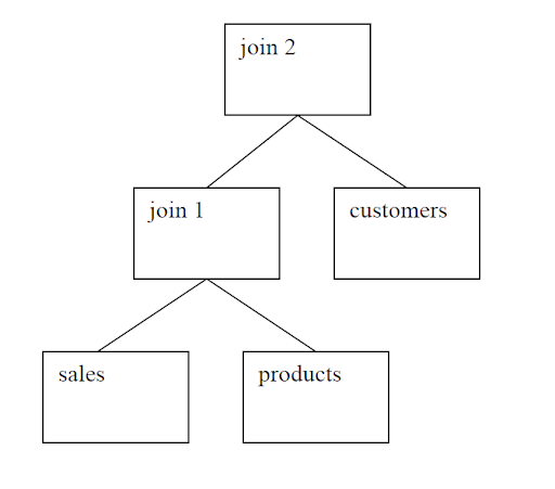
Join order 2:
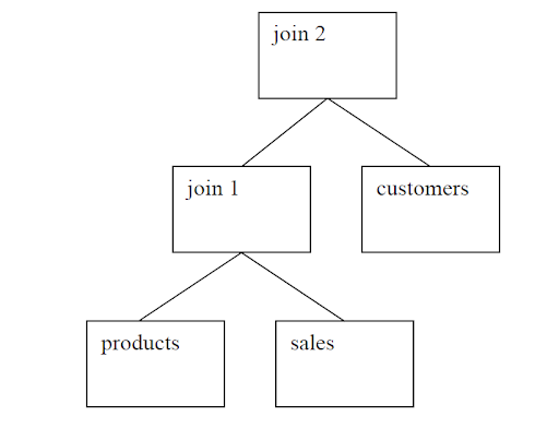
These differ because of asymmetry in the join methods. Typically a join will be more
efficient if the first table has fewer rows and the second has more. So, if you have more
sales rows and fewer products then the second join order would be faster if the join
method preferred fewer rows in the first table in the join.
Generally the best join order lists the tables in the order of the selectivity of their
predicates. If your query returns 1% of the sales rows and 50% of the products rows then
you probably should list sales before products in the join order. Let’s look at our
example query again:
select
sale_date, product_name, customer_name, amount
from sales, products, customers
where
sales.product_number=products.product_number and
sales.customer_number=customers.customer_number and
sale_date between
to_date('01/01/2012','MM/DD/YYYY') and
to_date('01/31/2012','MM/DD/YYYY') and
product_type = 'Cheese' and
customer_state = 'FL';
If your sales table has only January and February 2012 data in equal amounts then the
selectivity of the condition on sales_date is only 50%. If sales had ten years of equally
distributed data the selectivity would be less than 1%. You can easily determine the
selectivity by running two count(*) queries against the tables using the non-joining where
clause conditions:
products sales
join 1 customers
join 2
-- # selected rows
select
count(*)
from sales
where
sale_date between
to_date('01/01/2012','MM/DD/YYYY') and
to_date('01/31/2012','MM/DD/YYYY');
-- total #rows
select
count(*)
from sales;
You should do this for every table in the from clause to see the real selectivity.
In the same way, you need to know the selectivity of each subtree in the plan - i.e. each
combination of tables that have already been joined together. So, in our three table
example this would just be the three possible combinations - sales and products, sales and
customers, and customers and products. Here is the sales and products combination:
SQL> select count(*)
2 from sales, products
3 where
4 sales.product_number=products.product_number and
5 sale_date between
6 to_date('01/01/2012','MM/DD/YYYY') and
7 to_date('01/31/2012','MM/DD/YYYY') and
8 product_type = 'Cheese';
COUNT(*)
----------
4
SQL> select count(*)
2 from sales, products
3 where
4 sales.product_number=products.product_number;
COUNT(*)
----------
4
In this simple example the selectivity of the sales and products combination is 100%
because the count without the conditions against the constants equals the count with the
conditions with constants. But, in a real query these would differ and in some cases the
combination of conditions on two tables is much more selective than the conditions on
each individual table.
Extreme differences in selectivity cause reordering the joins to produce the best tuning
improvement. We started out this paper with the idea that you have a SQL statement that
is slow and you want to speed it up. You may want a query that runs for hours to run in
seconds. To find this kind of improvement by looking at join order and predicate
selectivity you have to look for a situation where the predicates on one of the tables has
an extremely high selectivity compared with the others. So, say your conditions on your
sales rows reduced the number of sales rows considered down to a handful of rows out of
the millions in the table. Putting the sales table first in the join order if it isn’t already put
there by the optimizer could produce a huge improvement, especially if the conditions on
the other large tables in the join were not very selective. What if your criteria for
products reduced you down to one product row out of hundreds of thousands? Put
products first. On the other hand if there isn’t a big gap in the selectivity against the
tables in the from clause then simply ordering the joins by selectivity is not guaranteed to
help.
You change the join order by giving the optimizer more information about the selectivity
of the predicates on the tables or by manually overriding the optimizer’s choice. If the
optimizer knows that you have an extremely selective predicate it will put the associated
table at the front of the join order. You can help the optimizer by gathering statistics on
the tables in the from clause. Accurate statistics help the optimizer know how selective
the conditions are. In some cases higher estimate percentages on your statistics gathering
can make the difference. In other cases histograms on the columns that are so selective
can help the optimizer realize how selective the conditions really are.
Here is how to set the optimizer preferences on a table to set the estimate percentage and
choose a column to have a histogram and gather statistics on the table:
-- 1 - set preferences
begin
DBMS_STATS.SET_TABLE_PREFS(NULL,'SALES','ESTIMATE_PERCENT','10');
DBMS_STATS.SET_TABLE_PREFS(NULL,'SALES','METHOD_OPT',
'FOR COLUMNS SALE_DATE SIZE 254 PRODUCT_NUMBER SIZE 1 '||
'CUSTOMER_NUMBER SIZE 1 AMOUNT SIZE 1');
end;
/
-- 2 - regather table stats with new preferences
execute DBMS_STATS.GATHER_TABLE_STATS (NULL,'SALES');
This set the estimate percentage to 10% for the sales table. It put a histogram on the
sales_date column only.
You can use a cardinality hint to help the optimizer know which table has the most
selective predicates. In this example we tell the optimizer that the predicates on the sales
table will only return one row:
SQL> select /*+cardinality(sales 1) */
2 sale_date, product_name, customer_name, amount
3 from sales, products, customers
4 where
5 sales.product_number=products.product_number and
6 sales.customer_number=customers.customer_number and
7 sale_date between
8 to_date('01/01/2012','MM/DD/YYYY') and
9 to_date('01/31/2012','MM/DD/YYYY') and
10 product_type = 'Cheese' and
11 customer_state = 'FL';
SALE_DATE PRODUCT_NAME CUSTOMER_NAME AMOUNT
--------- ------------ ----------------- ----------
04-JAN-12 Feta Sunshine State Co 300
02-JAN-12 Chedder Sunshine State Co 100
05-JAN-12 Feta Green Valley Inc 400
03-JAN-12 Chedder Green Valley Inc 200
Execution Plan
----------------------------------------------------------
0 SELECT STATEMENT Optimizer=ALL_ROWS
1 0 HASH JOIN
2 1 HASH JOIN
3 2 TABLE ACCESS (FULL) OF 'SALES' (TABLE)
4 2 TABLE ACCESS (FULL) OF 'PRODUCTS' (TABLE
5 1 TABLE ACCESS (FULL) OF 'CUSTOMERS' (TABLE)
As a result, the optimizer puts sales at the beginning of the join order. Note that in this
case for an example we lied to the optimizer since really there are four rows. Sometimes
giving the optimizer the true cardinality will work, but in others you will need to under or
overestimate to get the join order that is optimal.
You can use a leading hint to override the optimizer’s choice of join order. For example
if sales had the highly selective predicate you could do this:
SQL> select /*+leading(sales) */
2 sale_date, product_name, customer_name, amount
3 from sales, products, customers
4 where
5 sales.product_number=products.product_number and
6 sales.customer_number=customers.customer_number and
7 sale_date between
8 to_date('01/01/2012','MM/DD/YYYY') and
9 to_date('01/31/2012','MM/DD/YYYY') and
10 product_type = 'Cheese' and
11 customer_state = 'FL';
SALE_DATE PRODUCT_NAME CUSTOMER_NAME AMOUNT
--------- ------------ ----------------- ----------
04-JAN-12 Feta Sunshine State Co 300
02-JAN-12 Chedder Sunshine State Co 100
05-JAN-12 Feta Green Valley Inc 400
03-JAN-12 Chedder Green Valley Inc 200
Execution Plan
----------------------------------------------------------
0 SELECT STATEMENT Optimizer=ALL_ROWS
1 0 HASH JOIN
2 1 HASH JOIN
3 2 TABLE ACCESS (FULL) OF 'SALES' (TABLE)
4 2 TABLE ACCESS (FULL) OF 'PRODUCTS'
5 1 TABLE ACCESS (FULL) OF 'CUSTOMERS' (TABLE)
The leading hint on sales forced it to be the first table in the join order just like the
cardinality hint. It left it up to the optimizer to choose either products or customers as the
next table.
If all else fails and you can’t get the optimizer to join the tables together in an efficient
order you can break the query into multiple queries saving the intermediate results in a
global temporary table. Here is how to break our three table join into two joins - first
sales and products, and then the results of that join with customers:
SQL> create global temporary table sales_product_results
2 (
3 sale_date date,
4 customer_number number,
5 amount number,
6 product_type varchar2(12),
7 product_name varchar2(12)
8 ) on commit preserve rows;
Table created.
SQL> insert /*+append */
2 into sales_product_results
3 select
4 sale_date,
5 customer_number,
6 amount,
7 product_type,
8 product_name
9 from sales, products
10 where
11 sales.product_number=products.product_number and
12 sale_date between
13 to_date('01/01/2012','MM/DD/YYYY') and
14 to_date('01/31/2012','MM/DD/YYYY') and
15 product_type = 'Cheese';
4 rows created.
SQL> commit;
Commit complete.
SQL> select
2 sale_date, product_name, customer_name, amount
3 from sales_product_results spr, customers c
4 where
5 spr.customer_number=c.customer_number and
6 c.customer_state = 'FL';
SALE_DATE PRODUCT_NAME CUSTOMER_NAME AMOUNT
--------- ------------ ----------------- ----------
02-JAN-12 Chedder Sunshine State Co 100
03-JAN-12 Chedder Green Valley Inc 200
04-JAN-12 Feta Sunshine State Co 300
05-JAN-12 Feta Green Valley Inc 400
Breaking a query up like this is a very powerful method of tuning. If you have the ability
to modify an application in this way you have total control over how the query is run
because you decide which joins are done and in what order. I’ve seen dramatic run time
improvement using this simple technique.
JoinMethods
The choice of the best join method is determined by the number of rows being joined
from each source and the availability of an index on the joining columns. Nested loops
joins work best when the first table in the join has few rows and the second has a unique
index on the joined columns. If there is no index on the larger table or if both tables have
a large number of rows to be joined then hash join them with the smaller table first in the
join.
Here is our sample query’s plan with all nested loops:
Execution Plan
----------------------------------------------------------
0 SELECT STATEMENT Optimizer=ALL_ROWS
1 0 TABLE ACCESS (BY INDEX ROWID) OF 'CUSTOMERS' (TABLE)
2 1 NESTED LOOPS
3 2 NESTED LOOPS
4 3 TABLE ACCESS (FULL) OF 'SALES' (TABLE)
5 3 TABLE ACCESS (BY INDEX ROWID) OF 'PRODUCTS'
6 5 INDEX (RANGE SCAN) OF 'PRODUCTS_INDEX' (INDEX)
7 2 INDEX (RANGE SCAN) OF 'CUSTOMERS_INDEX' (INDEX)
In this example let’s say that the date condition on the sales table means that only a few
rows would be returned from sales. But, what if the conditions on products and
customers were not very limiting? Maybe all your customers are in Florida and you
mainly sell cheese. If you have indexes on product_number and customer_number or if
you add them then a nested loops join makes sense here.
But, what if the sales table had many rows in the date range the conditions on products
and customers were not selective either? In this case the nested joops join using the
index can be very inefficient. We have seen many cases were doing a full scan on both
tables in a join and using a hash join produces the fastest query runtime. Here is a plan
with all hash joins that we saw in our leading hint example:
Execution Plan
----------------------------------------------------------
0 SELECT STATEMENT Optimizer=ALL_ROWS
1 0 HASH JOIN
2 1 HASH JOIN
3 2 TABLE ACCESS (FULL) OF 'SALES' (TABLE)
4 2 TABLE ACCESS (FULL) OF 'PRODUCTS'
5 1 TABLE ACCESS (FULL) OF 'CUSTOMERS' (TABLE)
Of course you can mix and match and use a hash join in one case and nested loops in
another.
Execution Plan
----------------------------------------------------------
0 SELECT STATEMENT Optimizer=ALL_ROWS
1 0 TABLE ACCESS (BY INDEX ROWID) OF 'CUSTOMERS' (TABLE)
2 1 NESTED LOOPS
3 2 HASH JOIN
4 3 TABLE ACCESS (FULL) OF 'SALES' (TABLE)
5 3 TABLE ACCESS (FULL) OF 'PRODUCTS' (TABLE)
6 2 INDEX (RANGE SCAN) OF 'CUSTOMERS_INDEX' (INDEX)
As with join order you can cause the optimizer to use the optimal join method by either
helping it know how many rows will be joined from each row source or by forcing the
join method using a hint. The following hints forced the join methods used above:
/*+ use_hash(sales products) use_nl(products customers) */
Use_hash forces a hash join, use_nl forces a nested loops join. The table with the fewest
rows to be joined should go first. A great way to get the optimizer to use a nested loops
join is to create an index on the join columns of the table with the least selective where
clause predicates.
For example, these statements create indexes on the product_number
and customer_number columns of the products and customers tables:
create index products_index on products(product_number);
create index customers_index on customers(customer_number);
You can encourage hash joins by manually setting the hash_area_size to a large number.
The init parameter hash_area_size is an area of memory in each session’s server
process’s local memory (PGA) that buffers the on-disk hash table. The more memory
dedicated to hashing the more efficient a hash join is and the more likely the optimizer is
to choose a hash join over a nested loops join. You have to first turn off automatic pga
memory management by setting workarea_size_policy to manual and then setting sort
and hash area sizes.
Here is an example from a working production system:
NAME TYPE VALUE
------------------------------------ ----------- ---------
hash_area_size integer 100000000
sort_area_size integer 100000000
workarea_size_policy string MANUAL
Access Methods
For clarity we limit our discussion of access method to two options: index scan and full
table scan. There are many possible access methods but at its core the choice of access
method comes down to how many rows will be retrieved from the table. Access a table
using an index scan when you want to read a very small percentage of the rows,
otherwise use a full table scan. An old rule of thumb was that if you read 10% of the
table or less use an index scan. Today that rule should be 1% or even much less. If you
are accessing only a handful of rows of a huge table and you are not using an index then
switch to an index. If the table is small or if you are accessing even a modest percentage
of the rows you will want a full scan.
The parameters optimizer_index_caching, optimizer_index_cost_adj, and
db_file_multiblock_read_count all affect how likely the optimizer is to use an index
versus a full scan. You may find that you have many queries using indexes where a full
scan is more efficient or vice versa. These parameters can improve the performance of
many queries since they are system wide. On one Exadata system where we wanted to
discourage index use we set optimizer_index_cost_adj to 1000, ten times its normal
setting of 100. This caused many queries to begin using full scans, which Exadata
processes especially well. Here is the command we used to set this parameter value:
alter system set optimizer_index_cost_adj=1000 scope=both sid='*';
The greater the degree of parallelism set on a table the more likely the optimizer is to use
a full scan. So, if a table is set to parallel 8 the optimizer assumes a full scan takes 1/8th
the time it would serially. But there are diminishing marginal returns on increasing the
degree of parallelism. You get less benefit as you go above 8 and if you have many users
querying with a high degree of parallelism you can overload your system. This is how
you set a table to a parallel degree 8:
alter table sales parallel 8;
Last, but certainly not least in importance are index and full scan hints. Here are
examples of both:
/*+ full(sales) index(customers) index(products) */
These hints force the sales table to be accessed using a full scan, but require the
customers and products tables to be accessed using an index.
Conclusion
We have demonstrated how to tune an Oracle SQL query by examining and manipulating
the join order, join methods, and access methods used in the query’s execution plan. First
you must query the tables to determine the true number of rows returned from each table
and from each likely join. Then you identify which join order, join method, or access
method chosen by the optimizer is inefficient. Then you use one of the suggested
methods to change the optimizer’s choice to be the efficient one. These methods include
gathering optimizer statistics, hints, setting init parameters, breaking the query into
smaller pieces, and adjusting the parallel degree. Left unsaid is that you must test your
changed plan to make sure the new combination of join order, join methods and access
methods actually improve the performance. In SQL*Plus turn timing on and check the
elapsed time with the optimizer’s original execution plan and compare the elapsed time
with the new plan:
SQL> set timing on
SQL>
SQL> select
2 sale_date, product_name, customer_name, amount
3 from sales, products, customers
4 where
5 sales.product_number=products.product_number and
6 sales.customer_number=customers.customer_number and
7 sale_date between
8 to_date('01/01/2012','MM/DD/YYYY') and
9 to_date('01/31/2012','MM/DD/YYYY') and
10 product_type = 'Cheese' and
11 customer_state = 'FL';
SALE_DATE PRODUCT_NAME CUSTOMER_NAME AMOUNT
--------- ------------ ----------------- ----------
02-JAN-12 Chedder Sunshine State Co 100
03-JAN-12 Chedder Green Valley Inc 200
04-JAN-12 Feta Sunshine State Co 300
05-JAN-12 Feta Green Valley Inc 400
Elapsed: 00:00:00.00
This is the final test that our analysis has brought us to our initial goal - of vastly
improved run time for our problem query.

No comments:
Post a Comment